Survival analysis is a series of statistical methods that deals with variables that have both a time and event associated with it. For example, it is used in cancer clinical research if we are interested in measuring the time it takes before a patient relapses following treatment. In this case, the event we are measuring here is whether a patient relapses or not which has a time associated with when the relapse occurs.

This will be the first of several posts on this topic. In this first post, we will introduce survival analysis and basic concepts of it:

Table of Contents

What is Survival Analysis?

As mentioned in the introduction of this post, survival analysis is a series of statistical methods that deal with the outcome variable of interest being a time to event variable. This is unlike a typical regression problem where we might be working with a continuous outcome variable (e.g. housing price) or a classification problem where we simply have a discrete variable (e.g. Class I or Class II). In survival analysis, the outcome variable has both a event and a time value associated with it. Survival analysis is often used in medicine to study for instance a drug is able to prevent a disease from occurring (event) and how long it can say prevent it for (time). For the rest of this post, we will refer to time as survival time.

Censoring

One aspect that makes survival analysis difficult is the concept of censoring. What this means is that when a patient is censored we don’t know the true survival time for that patient. There are 3 main reasons why this happens:

1. Individual does not experience the event when the study is over.
2. Individual is lost to follow-up during the study period.
3. Individual withdraws from the study.

There are 3 major times of censoring: right, left and interval censoring which we will discuss below.

Right-censored

Right-censoring, the most common type of censoring, occurs when the survival time is “incomplete” at the right side of the follow-up period. Consider the follow example where we have 3 patients (A, B, C) enrolled onto a clinical study that runs for some period of time (study end - study start).

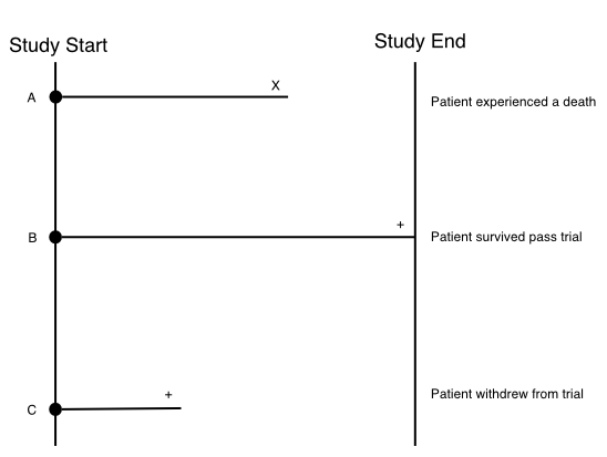
These 3 patients have three different trajectories:

1. Patient A: Experiences a death before the study ends. We count this as an event.
2. Patient B: Survives passed the end of the study.
3. Patient C: Withdraws from the study.

Patient A requires no censoring since we know their exact survival time which is the time until death. Patient B however neeeds to be censored (indicated with the + at the end of the follow-up time) since we don’t know the exact survival time of the patient; We only know that they survived up to at least the end of the study. Patient C also needs to be censored since they withdrew before the study ended. So we only know that they survived up to the time they withdrew, but again we don’t know the exact survival time of this patient. In right censoring, the true survival times will always be equal to or greater than the observed survival time.

Note: This example is a bit unrealistic since it’s rare to have all patients enrolled at the same time in a study. In reality, patients would be enrolled at different times in the trial. But this example is meant more so to illustrate the concepts of censoring.

Left-censored

In contrast to right-censoring, left censoring occurs when the person’s true survival time is less than or equal to the observed survival time. An example of a situation could be for virus testing. For instance, if we’ve been following an individual and recorded an event when for instance the individual tests positive for a virus:

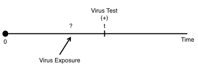
But we don’t know the exact time of when the individual was exposed to the disease. We only know that there was some exposure between 0 and the time they were tested:

Interval-censored

Using the virus testing example, if we have the situation whether we’ve performed testing on the indvidual at some timepoint ($t_{1}$) and the individual was negative. But then at a timepoint further on ($t_{2}$), the individual tested positive:

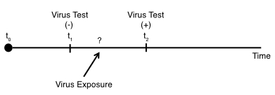
In this scenario, we know the individual was exposed to the virus sometime between $t_{1}$ and $t_{2}$, but we do not know the exact timing of the exposure.

Terminology

Before going further on in this post, it’s a good time to introduce some key terminology and mathematical notation in survival analysis. The first one is:

T

Random variable for a person’s survival time.

As T denotes time, it can take on any value between 0 to infinity. We then use:

t

Specific value of interest for random variable T.

So the notation, $T > t = 2)$, means we are asking whether the individual had a survival time beyond 2 months (if the unit of time is months).

d

Random variable indicating an event or censorship.

So for instance, we could encode events as a 1 and thus d = 1 represents the situation where an event occurs during study period. Where as d = 0, survival time is censored by end of the study.

Next there are two quantitative functions which are of interest in survival analysis. These are the survivor function and hazard function.

Survivor Function

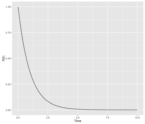
The survivor function (aka. survival function, reliability function) is denoted as $S(t)$. The survivor function gives the probability that a person survives longer than some specific time t $S(t) = P(T > t)$. All survivor functions follow these same 3 characteristics:

• As t increases, the $S(t)$ should decrease.
• $S(0) = 1$. That is at the start of the study, no one has the event and hence the probability of surviving at $t = 0$ is 1.
• $S(\infty) = 0$. If the study were to go to $S(\infty)$, then everyone will eventually experience the event and hence the survival probability must be 0.

In theory, survival curves should be a “smooth” function with time ranging from 0 to $\infty$:

library("dplyr")
library("ggplot2")

data.frame(x = c(0, 10)) %>%
  ggplot(aes(x = x)) +
  stat_function(fun = dexp, args = list(rate = 1)) +
  ylab("S(t)") +
  xlab("Time")

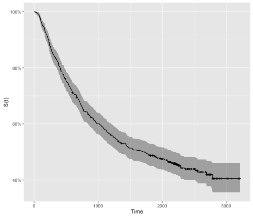
However, it is typical to empirically derive the survivor function from data using what is called the Kaplan-Meier method (we will cover this in an additional post). As we are often dealing with small cohorts, the survival curves oftne come out with lots of “steps”:

library("survival")
library("ggfortify")

colon.survfit <- 
  colon %>%
  filter(rx == "Obs") %>%
  survfit(Surv(time, status) ~ 1, data = .)

colon.survfit %>%
  autoplot() +
  ylab("S(t)") +
  xlab("Time")

Hazard Function

The other quantitative function of interest in survival analysis is the hazard function, $h(t)$. I always found the hazard function a bit difficult to intepret. The easiest way to think about it is to consider the scenario of where you are reading off a speedometer at a specific moment $t$. At this specific moment, the speed you are travelling at is 40 km/hr. What this means is if you travel at this specific rate for the next hour, you will travel 40 kilometers. But of course, there will be flucuations and you will go faster or slower than 40 km/hr so it doesn’t really give you the specific distance you will travel. So what does the 40km/hr really mean then? All it tells you is at this given moment you are travelling this fast. Importantly, implicit to this is the fact that you have already travelled some amount of distance.

The hazard function is akin to the speedometer here. Where at given moment t in time, you have this potential risk of having an event given you have survived up to time t. Mathematically, $h(t)$ is represented as follows:

Let’s break down this equation:

• $\lim_{\Delta t\to\infty}$: This indicates as the time interval approaches 0. This essentially gives us the instantaneous measurement at a particular time.
• $P(t \leq T < t + \Delta t\ |\ T \geq t)$: Probability that a person’s survival time T will be between the time interval $t$ and $t + \Delta t$ given that they have survived up to t ($T \geq t$).

So what this equation is telling us is if the time interval approaches 0 ($\lim_{\Delta t\to\infty}$), then we are getting the instantaneous risk of having an event at time t given they have survived up to t.

It’s important to note here that the hazard is not a probability because we are dividing the probability by a time interval. Instead what we get is a rate. And since we are dealing with the condition of survival up to time t, this is why sometimes the hazard function is referred to as conditional failure rate.

Unlike the $S(t)$, estimating the $h(t)$ is not as simple. One approach to estimating $h(t)$, is to first estimate the cumulative hazard function $H(t)$ which is used as an intermediary to estimating $h(t)$. The Nelson–Aalen estimator can be used to first estimate $H(t)$ and then calculate the hazard function from that.

library("muhaz")
library("magrittr")

# Uses Nelson-Aalen estimator to first get cumulative hazard, and then predict
# the hazard function from that.
colon.kphaz.fit <- 
  colon %>%
  filter(rx == "Obs") %$%
  kphaz.fit(.$time, .$status, method = "nelson")

colon.kphaz.fit %>%
  as.data.frame() %>%
  ggplot(aes(x = time, y = haz)) +
  geom_line() +
  xlab("Time") +
  ylab("h(t)")

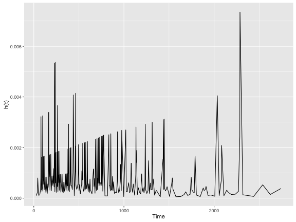
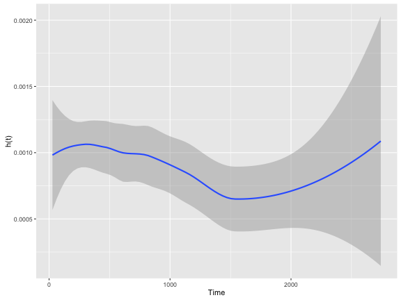
As you can see, the $h(t)$ is fairly erratic which is common. A “smoothing” line is often drawn to help make it more intepretable.

colon.kphaz.fit %>%
  as.data.frame() %>%
  ggplot(aes(x = time, y = haz)) +
  geom_smooth() +
  xlab("Time") +
  ylab("h(t)")

Like $S(t)$, $h(t)$ has a few key properties:

• It is always non-negative.
• It has no upper bound. In other words, unlike $S(t)$, which is a probability, the $h(t)$ can be > 1 and can go up to $\infty$.

It is worth mentioning that if we assume $h(t)$ (and $S(t)$) follow a probability distribution then we can also esimate the functions this way. We will discuss this in a later post.

Survivor Function vs. Hazard Function

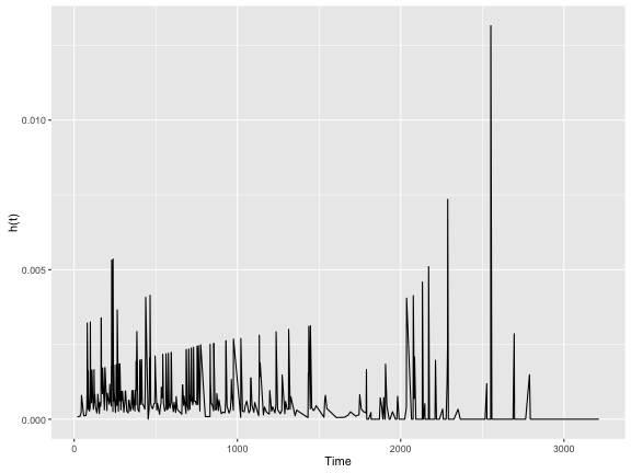
An important thing to mention is that $S(t)$ and $h(t)$ are related through these two formulas:

We can make sure of statistical computing languages (e.g. R) to make us make these transformations. For instance, the epiR package in R has the epi.insthaz function which can transform $S(t)$ into a $h(t)$:

library("epiR")

colon.haz <- epi.insthaz(colon.survfit, conf.level = 0.95)
colon.haz %>%
  ggplot(aes(x = time, y = est)) +
  geom_line() +
  ylab("h(t)") +
  xlab("Time")

Summary

Hopefully this first post on survival analysis gave you a good idea of some of the basic concepts in survival analysis. Ultimately, there are 3 major goals in survival analysis:

1. Estimate the survivor and hazard functions.
2. Compare survivor and/or hazard functions (e.g. log-rank test)
3. Assess the relationship of other variables with the survivor and hazard function. (e.g. cox regression)

We will cover each of these topics in more details in subsequent posts. So stay tuned!

References

• Survival Analysis - A Self Learning Text
• Survival Analysis Part I: Basic concepts and first analyses
• Nelson-Aalen estimator in R
• Nelson-Aalen estimator of cumulative hazard