Probability Distributions and their Mass/Density Functions
: R, Statistics
A probability distribution is a way to represent the possible values and the respective probabilities of a random variable. There are two types of probability distributions: discrete and continuous probability distribution. As you might have guessed, a discrete probability distribution is used when we have a discrete random variable. A continuous probability distribution is used when we have a continuous random variable.
In this post, we will explore what discrete and continuous probability distributions are. Additionally, we will describe what a probability mass and density function, their key properties, and how they relate to probability distributions. Here is an overview of what will be discussed in this post.
Table of Contents
Discrete Probability Distributions
In my previous post on random variables, I used the example of a random process that involved flipping a coin x number of times and measuring the total number of heads using a discrete random variable X. As an example, let us try to build a probability distribution from a random process like this where we are flipping a coin 3 times. This random process can have a total of 8 possible outcomes:
Heads Up!
[I suggest watching this video](https://www.youtube.com/watch?v=5lpqiGixDd0) if you are unclear on how these outcomes were generated.- HHH
- HHT
- HTH
- HTT
- THH
- THT
- TTH
- TTT
We let our random variable Y serve as a way to map the number of heads we get to a numeric value. So the most initutive way would be:
- X = 0 if we get no heads.
- X = 1 if we get 1 head.
- X = 2 if we get 2 heads.
- X = 3 if we get 3 heads.
So now that we have this random variable and the possible values this variable can take, let’s try to figure out the associated probabilities of each outcome.
- $P(X = 0)$: The only way we can get 0 heads is if all 3 coin flips gives a tail. The only outcome that satisfies this is the TTT outcome. This means the probability $P(X = 0) = \frac{1}{8}$.
- $P(X = 1)$: To get 1 head, the outcomes HTT, THT, and TTH satisfy this. So this means $P(X = 1) = \frac{3}{8}$.
- $P(X = 2)$: To get 2 heads, the outcomes HHT, HTH, and THH satisfy this. So this means $P(X = 2) = \frac{3}{8}$.
- $P(X = 3)$: The only way we can get 3 heads is if all 3 coin flips gives a head The only outcome that satisfies this is the TTT outcome. This means the probability $P(X = 3) = \frac{1}{8}$.
What we have just described is called a “probability mass function (pmf)” which is a function, $f(X)$, that defines the probability of the discrete random variable X taking on a particular value x. When we take all the possible values (sample space) and associated probabilities into consideration, it is called a discrete probability distribution (as defined by a pmf). We can visualize this particular pmf as follows:
library("ggplot2")
library("dplyr")

prob.distr.df <- data_frame(value = c(0, 1, 2, 3),
                            prob = c(1/8, 3/8, 3/8, 1/8))

prob.distr.df %>%
  ggplot(aes(x = value, y = prob)) +
  geom_bar(stat = "identity") +
  ylim(c(0, 1)) +
  xlab("X (Number of Heads)") +
  ylab("f(X) Probability")

Here we have a discrete probability distribution of the random variable Y. The x-axes shows the different outcomes of the random variable while the y-axes shows the corresponding probabilities of these outcomes
You might sometimes see the term probability distribution table. This is just the same thing as a pmf. The name stems from the fact that there are a finite number of outcomes and and so we can represent these outcomes and their associated probabilities in a finite table. As we will see below, we can’t do this for a continuous random variable hence why a probabilty distribution table only has meaning in the context of a discrete random variable.
Continuous Probability Distributions
In the example above, X was a discrete random variable. When the outcomes are discrete we have the ability to directly measure the probability of each outcome. When the random variable is continuous, then things get a little more complicated. We are not able to directly measure the probability of a specific continuous value. This may seem a bit confusing at first, but imagine you had a random variable, Y, that measured the price of a diamond. Now what if someone asked you the following question: If you sampled a single diamond, what is the probability that its exact price is $326.57? Not $326.58 or $326.56, but exactly $326.57?
If you think of it that way, then the probability of getting a diamond with that exact price is probably really low. In fact, the probability of any exact price is really low. This is why the concept of probability for a given value when the value is on a continous scale doesn’t make sense. Instead, what we do is “discretize” the sample space so that we can work in intervals instead of individual values. To make this more concrete, we will use the diamond dataset from ggplot2 to illustrate this example. First, let’s plot a summary histogram of the diamond prices for 53940 diamonds and use an interval size of 100 (to represent $100 intervals):
diamonds %>%
  ggplot(aes(x = price)) +
  geom_histogram(binwidth = 100) +
  xlab("Y (Diamond Price)") +
  ylab("Number of Diamonds")

Once we have these intervals of data, we can start talking about proportion of samples falling into intervals For instance, we can ask the question what is the probability of a diamond having a price between $1000 and $1100:
num.diamonds.in.bin <-
  diamonds %>%
  filter(price > 1000, price < 1100) %>%
  nrow()
A total of 1832 diamonds fall in this interval which equates to the following proportion of all diamonds in the dataset:
prob.mass <- num.diamonds.in.bin / nrow(diamonds)
prob.mass
## [1] 0.03396366
When we talk about the proportion of outcomes falling into an interval like this, then this is called a “probability mass”. As the probability mass is dependent on the interval size, the “probability density” is used to represent the ratio of the probability mass to interval size:
prob.dens <- prob.mass / 100
prob.dens
## [1] 0.0003396366
To get more precision, we would want our intervals to be small since wide intervals are not very informative. Ideally, our intervals should be infinitesimally small. When we do this, we produce something that starts to resemble a “curve” (here we use kernel density estimation to estimate the curve).
diamonds %>%
  ggplot(aes(x = price)) +
  geom_density() +
  xlab("Y (Diamond Price)") +
  ylab("f(Y) Density")

This “curve”, $f(Y)$, is called a probability density function (pdf) which is used to describe the probability distribution of a continuous random variable.
Properties of Probability Mass/Density Functions
There are a few key properites of a pmf, $f(X)$:
-
$f(X = x) > 0$ where $x \in S_{X}$ ($S_{X}$ = sample space of X).
-
Since we can directly measure the probability of an event for discrete random variables, then
$$P(X = x) = f(X = x)$$ -
The probability of all possible events must sum to 1:
$$\sum_{x \in S_{X}} f(X) = 1$$
The key properites of a pdf, $f(Y)$, are very similar to a pmf. The big difference is that we need to think in terms of intervals instead of individual outcomes. This means we have to work with integrals and not summations:
-
$f(Y = y) > 0$ where $y \in S_{Y}$ ($S_{Y}$ = sample space of Y). This property is the same as for a pmf.
-
The probability of a value $y \in [a, b]$ is:
$$P(a \leq y \leq b) = \int_{a}^{b} f(Y) \,dy$$In other words, the probability of $y \in [a, b]$ is equivalent to taking the integral of the pdf between a and b.
-
The entire area under the pdf must sum to 1.
$$\int_{-\infty}^{\infty} f(Y) \,dy = 1$$
Types of Probability Mass/Density Functions
You may have heard the phrase that random variable “Y follows a [insert name of] distribution”. What this means is that they are assuming the data being generated comes from a particular well studied distribution. In statistics, there exists many discrete (e.g. binomial, negative binomial) and continuous (e.g. gaussian, student-t) distributions that have been well studied. So by making the assumption that a random variable follows a particular distribution, we can use the distribution’s derived pmf/pdf and established properties to help us answer questions about the data. For instance, we know that the pdf of a gaussian is:
It is parameterized by a mean $\mu$ and a standard deviation $\sigma$ while being symmetrical around the mean. A standard gaussian ($\mu = 0, \sigma = 1$) would look like this.
set.seed(1)

vals <- rnorm(200)

# dnorm provides the probability density
data.frame(x = vals) %>%
  ggplot(aes(x = vals)) +
  stat_function(fun = dnorm) +
  ylab("Density")

Just like before, we can ask questions like $P(-2 \leq y \leq 2)$ and use the gaussian pdf to answer this question:
# pnorm provides the probability
pnorm(2) - pnorm(-2)
## [1] 0.9544997
pnorm(y) function is essentially taking the integral from $-\infty$ to $y$:
So what we are doing here is:
This effectively calculates the area between -2 and 2:
# dnorm provides the probability density
data.frame(x = vals) %>%
  ggplot(aes(x = vals)) +
  stat_function(fun = dnorm) +
  ylab("Density") +
  geom_vline(xintercept = -2, linetype = "dotted", color = "red") +
  geom_vline(xintercept = 2, linetype = "dotted", color = "red")

One caveat of this approach is that our assumption could be wrong. This means that one needs to be careful when deciding what type of probability distribution a random variable follows.
Thankfully there are some well established principles that can help us. The figure below provides a decision tree that gives you an idea of some common probability distributions that one can use given the data they have in hand:
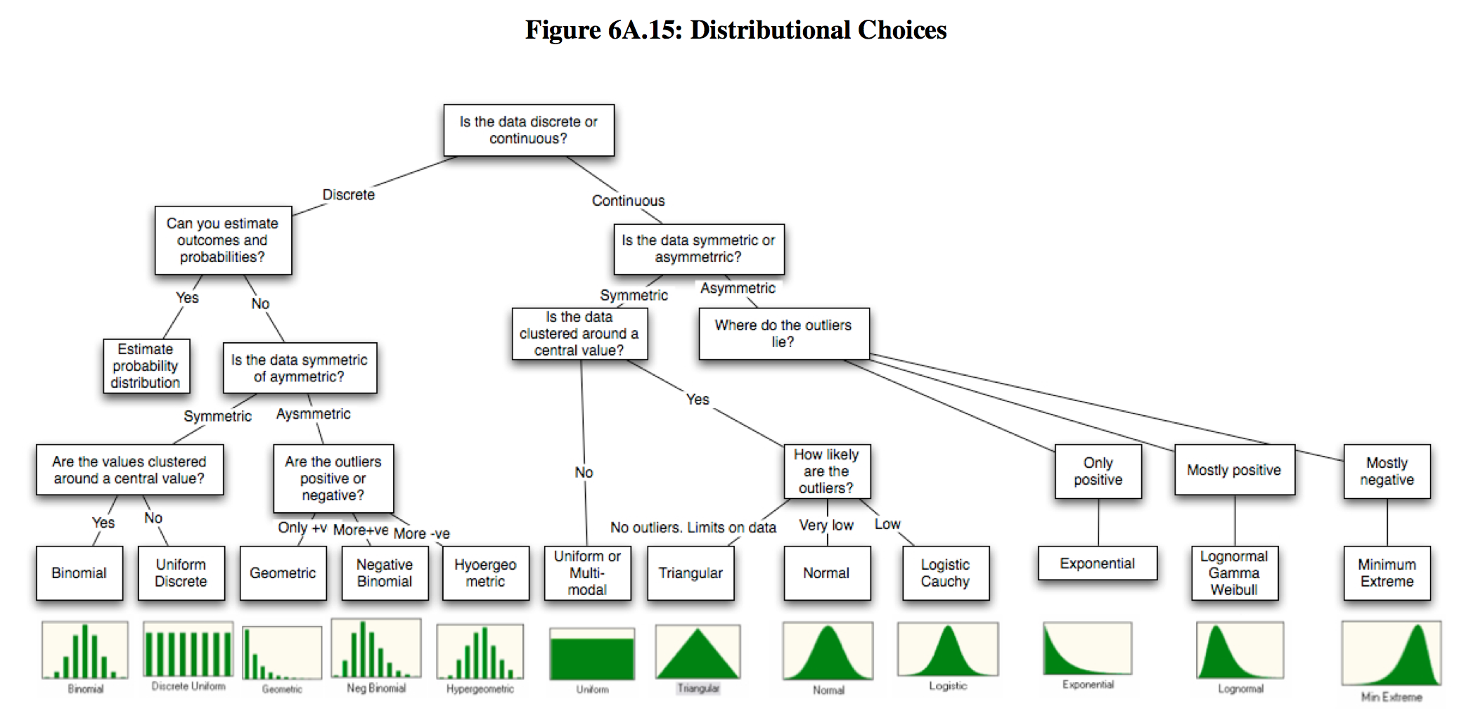
This is Figure 6A.15 (Pg 61) from Probabilistic approaches to risk by Aswath Damodaran.
Summary
Hopefully this post sheds a bit of light on what a probability distribution and how we can describe them using probability mass/density functions. The big take home messages are as follows:
- A probability distribution is a way to represent the possible values and the respective probabilities of a random variable. There are two types of probability distributions:
- Discrete probability distribution for discrete random variables.
- Continuous probability distribution for continuous random variables.
- We can directly calculate probabilites of a discrete random variable, X = x, as the proportion of times the x value occurs in the random process.
- Probabilites of a continuous random variable taking on a specific value (e.g. Y = y) are not directly measureable. Instead, we calculate the probability as the proportion of times $y \in [a, b]$.
- Probability mass functions (pmf) are used to describe discrete probability distributions. While probability density functions (pdf) are used to describe continuous probability distributions.
- By assuming a random variable follows an established probability distribution, we can use its derived pmf/pdf and established principles to answer questions we have about the data.
References
- Doing Bayesian Data Analysis - A Tutorial with R, JAGS, and Stan
- Probability Distribution Table - Intro with tossing a coin 3 times
- What is a Probability Distribution?
- Continuous Probability Distribution
- Khan Academy - Probability density function
- PennState STAT 414/415 - Probability Density Functions
- What is the relationship between the probability mass, density, and cumulative distribution functions?
R Session
devtools::session_info()
## Session info --------------------------------------------------------------
##  setting  value
##  version  R version 3.2.2 (2015-08-14)
##  system   x86_64, darwin13.4.0
##  ui       unknown
##  language (EN)
##  collate  en_CA.UTF-8
##  tz       America/Vancouver
##  date     2016-03-18
## Packages ------------------------------------------------------------------
##  package    * version    date       source
##  argparse   * 1.0.1      2014-04-05 CRAN (R 3.2.2)
##  assertthat   0.1        2013-12-06 CRAN (R 3.2.2)
##  captioner  * 2.2.3.9000 2015-09-16 local
##  colorspace   1.2-6      2015-03-11 CRAN (R 3.2.2)
##  DBI          0.3.1      2014-09-24 CRAN (R 3.2.2)
##  devtools     1.9.1      2015-09-11 CRAN (R 3.2.2)
##  digest       0.6.9      2016-01-08 CRAN (R 3.2.2)
##  dplyr      * 0.4.3      2015-09-01 CRAN (R 3.2.2)
##  evaluate     0.8        2015-09-18 CRAN (R 3.2.2)
##  findpython   1.0.1      2014-04-03 CRAN (R 3.2.2)
##  formatR      1.2.1      2015-09-18 CRAN (R 3.2.2)
##  getopt       1.20.0     2013-08-30 CRAN (R 3.2.2)
##  ggplot2    * 2.0.0      2015-12-18 CRAN (R 3.2.2)
##  gtable       0.1.2      2012-12-05 CRAN (R 3.2.2)
##  knitr      * 1.12.7     2016-02-09 local
##  labeling     0.3        2014-08-23 CRAN (R 3.2.2)
##  lazyeval     0.1.10     2015-01-02 CRAN (R 3.2.2)
##  magrittr   * 1.5        2014-11-22 CRAN (R 3.2.2)
##  memoise      0.2.1      2014-04-22 CRAN (R 3.2.2)
##  munsell      0.4.3      2016-02-13 CRAN (R 3.2.2)
##  plyr         1.8.3      2015-06-12 CRAN (R 3.2.2)
##  proto      * 0.3-10     2012-12-22 CRAN (R 3.2.2)
##  R6           2.1.2      2016-01-26 CRAN (R 3.2.2)
##  Rcpp         0.12.3     2016-01-10 CRAN (R 3.2.2)
##  rjson        0.2.15     2014-11-03 CRAN (R 3.2.2)
##  scales       0.3.0      2015-08-25 CRAN (R 3.2.2)
##  stringi      1.0-1      2015-10-22 CRAN (R 3.2.2)
##  stringr      1.0.0      2015-04-30 CRAN (R 3.2.2)