Using Mixture Models for Clustering
: Mixture Models, R
If you’ve been exposed to machine learning in your work or studies, chances are you’ve heard of the term mixture model. But what exactly is a mixture model and why should you care?
A mixture model is a mixture of k component distributions that collectively make a mixture distribution $f(x)$:
The $\alpha_{k}$ represents a mixing weight for the $k^{th}$ component where $\sum_{k=1}^{K}\alpha_{k} = 1$. The $f_k(x)$ components in principle are arbitrary in the sense that you can choose any sort of distribution. In practice, parametric distribution (e.g. gaussians), are often used since a lot work has been done to understand their behaviour. If you substitute each $f_k(x)$ for a gaussian you get what is known as a gaussian mixture models (GMM). Likewise, if you substitute each $f_k(x)$ for a binomial distribution, you get a binomial mixture model (BMM). Since each parametric distribution has it’s own parameters, we can represent the parameters of each component with a $\theta_{k}$:
Why Would You Use a Mixture Model?
Let’s motivate the reason of why you woud use a mixture model by using an example. Let’s say someone presented you with the following density plot:
library("ggplot2")
library("dplyr")

options(scipen = 999)

p <- ggplot(faithful, aes(x = waiting)) +
  geom_density()
p
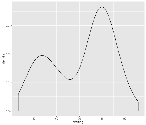
We can immediately see that the resulting distribution appears to be bi-modal (i.e. there are two bumps) suggesting that these data might be coming from two different sources. These data are actually from the faithful dataset available in R:
head(faithful)
##   eruptions waiting
## 1     3.600      79
## 2     1.800      54
## 3     3.333      74
## 4     2.283      62
## 5     4.533      85
## 6     2.883      55
This data is 2-column data.frame
- eruptions: Length of eruption (in mins)
- waiting: Time in between eruptions (in mins)
Putting the data into context suggests that the eruption times may be coming from two different subpopulations. There could be several reasons for this. For instance, maybe at different times of the year the geyser eruptions are more frequent. You can probably take an intutive guess as to how you could split this data.
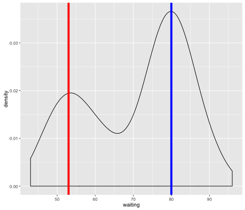
For instance, there likely is a subpopulation with a mean eruption of ~53 with some variance around this mean (red vertical line in figure below.) Another population with a mean eruption of ~80 with again some variance around this mean (blue vertical line in figure below).
p +
  geom_vline(xintercept = 53, col = "red", size = 2) +
  geom_vline(xintercept = 80, col = "blue", size = 2)
In fact, what we’ve done is a naive attempt at trying to group the data into subpopulations/clusters. But surely there must be some objective and “automatic” way of defining these clusters? This is where mixture models come in by providing a “model-based approach” to clustering through the use of statistical distributions. In the next section, we will utilize an R package to perfom some mixture model clustering.
Using a Gaussian Mixture Model for Clustering
As mentioned in the beginning, a mixture model consist of a mixture of distributions. The first thing you need to do when performing mixture model clustering is to determine what type of statistical distribution you want to use for the components. For this post, we will use one of the most common statistical distributions used for mixture model clustering which is the Gaussian/Normal Distribution:
\[\mathcal{N}(\mu, \sigma^2)\]The normal distribution is parameterized by two variables:
- $\mu$: Mean; Center of the mass
- $\sigma^2$: Variance; Spread of the mass
When Gaussians are used for mixture model clustering, they are referred to as Gaussian Mixture Models (GMM). As it turns out, our earlier intuition on where the means and variance of the subpopulation in the plot above is a perfect example of how we could apply a GMM. Specifically, we could try to represent each subpopulation as its own distribution (aka. mixture component). The entire set of data could then be represented as a mixture of 2 Gaussian distributions (aka. 2-component GMM)
In R, there are several packages that provide an implementation of GMM already (e.g. mixtools, mclust). As there exists a nice blog post by Ron Pearson on using mixtools on the faithful dataset, we will just borrow a bit his code to demonstrate the GMM in action:
library("mixtools")

#' Plot a Mixture Component
#'
#' @param x Input data
#' @param mu Mean of component
#' @param sigma Standard deviation of component
#' @param lam Mixture weight of component
plot_mix_comps <- function(x, mu, sigma, lam) {
  lam * dnorm(x, mu, sigma)
}

set.seed(1)
wait <- faithful$waiting
mixmdl <- normalmixEM(wait, k = 2)
## number of iterations= 29
data.frame(x = mixmdl$x) %>%
  ggplot() +
  geom_histogram(aes(x, ..density..), binwidth = 1, colour = "black",
                 fill = "white") +
  stat_function(geom = "line", fun = plot_mix_comps,
                args = list(mixmdl$mu[1], mixmdl$sigma[1], lam = mixmdl$lambda[1]),
                colour = "red", lwd = 1.5) +
  stat_function(geom = "line", fun = plot_mix_comps,
                args = list(mixmdl$mu[2], mixmdl$sigma[2], lam = mixmdl$lambda[2]),
                colour = "blue", lwd = 1.5) +
  ylab("Density")
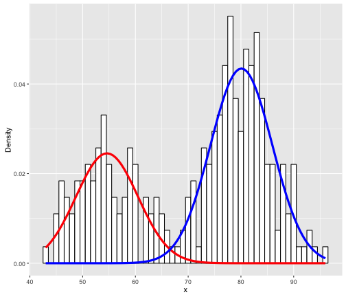
The key is the normalmixEM function which builds a 2-component GMM (k = 2 indicates to use 2 components). So how do we interpret this? It’s actually quite simply; The red and blue lines simply indicate 2 different fitted Gaussian distributions. Specifically, the means of the 2 Gaussians (red and blue) are respectively:
mixmdl$mu
## [1] 54.61489 80.09109
With respectively standard deviations of:
mixmdl$sigma
## [1] 5.871244 5.867716
You might also notice how the “heights” of the two components (herein we will refer to distribution as component) are different. Specifically, the blue component is “higher” than the red component. This is because the blue component encapsulates more density (i.e. more data) compared to the red component. How much exactly? You can get this value by using:
mixmdl$lambda
## [1] 0.3608869 0.6391131
Formally, these are referred to as the mixing weights (aka. mixing proportions, mixing coefficients). One can interpret this as the red component representing 36.089% and the blue component representing 63.911% of the input data. Another important aspect is that each input data point is actually assigned a posterior probability of belonging to one of these components. We can retrieve these data by using the following code:
post.df <- as.data.frame(cbind(x = mixmdl$x, mixmdl$posterior))
head(post.df, 10)  # Retrieve first 10 rows
##     x          comp.1         comp.2
## 1  79 0.0001030875283 0.999896912472
## 2  54 0.9999093397312 0.000090660269
## 3  74 0.0041357268361 0.995864273164
## 4  62 0.9673819082244 0.032618091776
## 5  85 0.0000012235720 0.999998776428
## 6  55 0.9998100114503 0.000189988550
## 7  88 0.0000001333596 0.999999866640
## 8  85 0.0000012235720 0.999998776428
## 9  51 0.9999901530788 0.000009846921
## 10 85 0.0000012235720 0.999998776428
The x column indicates the value of the data while comp.1 and comp.2 refers to the posterior probability of belonging to either component respectively. If you look at the x value in the first row, 79, you will see that it sits pretty close to the middle of the blue component (the mean of the blue component 80.091). So it makes sense that the posterior of this data point belonging to this component should be high (0.9999 vs. 0.0001). And simiarly, the data that sits inbetween the two components will have posterior probabilities that are not strongly associated with either component:
post.df %>%
  filter(x > 66, x < 68)
##    x    comp.1    comp.2
## 1 67 0.4235423 0.5764577
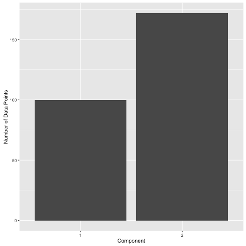
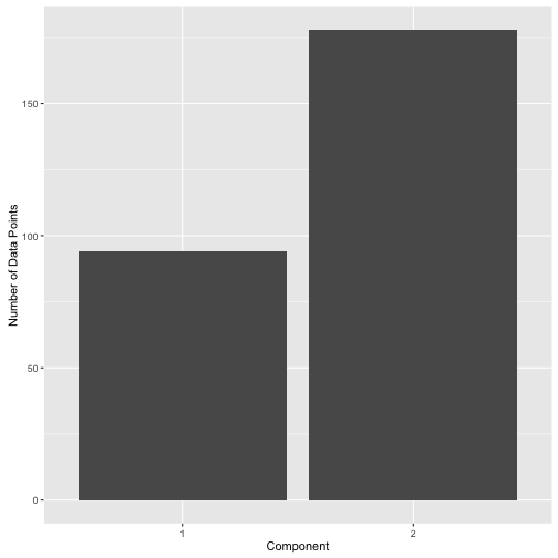
It’s important to understand that no “labels” have been assigned here actually. Unlike k-means which assigns each data point to a cluster (defined as a “hard-label”), mixture models provide what are called “soft-labels”. The end-user decides on what “threshold” to use to assign data into the components. For instance, one could use 0.3 as posterior threshold to assign data to comp.1 and get the following label distribution.
post.df %>%
  mutate(label = ifelse(comp.1 > 0.3, 1, 2)) %>%
  ggplot(aes(x = factor(label))) +
  geom_bar() +
  xlab("Component") +
  ylab("Number of Data Points")
Or one could use 0.8 and get the following label distribution:
post.df %>%
  mutate(label = ifelse(comp.1 > 0.8, 1, 2)) %>%
  ggplot(aes(x = factor(label))) +
  geom_bar() +
  xlab("Component") +
  ylab("Number of Data Points")
Summary
As you’ll seen from the above example, the usage of mixture model clustering can be very powerful in providing an objective way to clustering data. Some benefits to using mixture model clustering are:
- Choice of Component Distribution: In this post, we’ve used a gaussian distribution for each component. But we are not limited to using just gaussians. We can use binomials, multinomials, student-t, and other types of distributions depending on the type of data we have. We can even mix together different types of distributions. For example, it is common to GMM with an additional uniform distribution to capture any outlier data points.
- “Soft Labels”: There are no “hard” labels in mixture model clustering. Instead what we get is a probability of a data point belonging each component. Ultimately, the end-user decides on the probability threshold to assign a data point to a cluster creating what are called “soft” labels.
- Density Estimation: We get a measure how much data each component represents through the mixing weights.
If you are like me, you might be interested in knowing what is happening “under the hood”. In a subsequent post, I will walk through the math and show how you can implement your very own mixture model in R. So stay tuned!
References
R Session
devtools::session_info()
## Session info --------------------------------------------------------------
##  setting  value
##  version  R version 3.2.2 (2015-08-14)
##  system   x86_64, darwin11.4.2
##  ui       unknown
##  language (EN)
##  collate  en_CA.UTF-8
##  tz       America/Vancouver
##  date     2017-01-13
## Packages ------------------------------------------------------------------
##  package    * version date       source
##  argparse   * 1.0.1   2014-04-05 CRAN (R 3.2.2)
##  assertthat   0.1     2013-12-06 CRAN (R 3.2.2)
##  boot         1.3-17  2015-06-29 CRAN (R 3.2.2)
##  colorspace   1.2-6   2015-03-11 CRAN (R 3.2.2)
##  DBI          0.3.1   2014-09-24 CRAN (R 3.2.2)
##  devtools     1.9.1   2015-09-11 CRAN (R 3.2.2)
##  digest       0.6.9   2016-01-08 CRAN (R 3.2.2)
##  dplyr      * 0.4.3   2015-09-01 CRAN (R 3.2.2)
##  evaluate     0.8     2015-09-18 CRAN (R 3.2.2)
##  findpython   1.0.1   2014-04-03 CRAN (R 3.2.2)
##  formatR      1.2.1   2015-09-18 CRAN (R 3.2.2)
##  getopt       1.20.0  2013-08-30 CRAN (R 3.2.2)
##  ggplot2    * 2.1.0   2016-03-01 CRAN (R 3.2.2)
##  gtable       0.1.2   2012-12-05 CRAN (R 3.2.2)
##  knitr      * 1.13    2016-05-09 CRAN (R 3.2.2)
##  labeling     0.3     2014-08-23 CRAN (R 3.2.2)
##  lazyeval     0.1.10  2015-01-02 CRAN (R 3.2.2)
##  magrittr     1.5     2014-11-22 CRAN (R 3.2.2)
##  MASS         7.3-45  2015-11-10 CRAN (R 3.2.2)
##  memoise      0.2.1   2014-04-22 CRAN (R 3.2.2)
##  mixtools   * 1.0.4   2016-01-12 CRAN (R 3.2.2)
##  munsell      0.4.2   2013-07-11 CRAN (R 3.2.2)
##  nvimcom    * 0.9-14  2017-01-13 local
##  plyr         1.8.3   2015-06-12 CRAN (R 3.2.2)
##  proto      * 0.3-10  2012-12-22 CRAN (R 3.2.2)
##  R6           2.1.1   2015-08-19 CRAN (R 3.2.2)
##  Rcpp         0.12.2  2015-11-15 CRAN (R 3.2.2)
##  rjson        0.2.15  2014-11-03 CRAN (R 3.2.2)
##  scales       0.3.0   2015-08-25 CRAN (R 3.2.2)
##  segmented    0.5-1.4 2015-11-04 CRAN (R 3.2.2)
##  stringi      1.0-1   2015-10-22 CRAN (R 3.2.2)
##  stringr      1.0.0   2015-04-30 CRAN (R 3.2.2)