I recently had a chance to try out the TrAp software from the Yuval Kluger’s Lab:

Strino, F., Parisi, F., Micsinai, M., & Kluger, Y. (2013). TrAp: a tree approach for fingerprinting subclonal tumor composition. Nucleic Acids Res, 41(17), e165–e165

TrAP is an algorithm for inferring the “composition, abundance and evolutionary paths of the underlying cell subpopulations of a tumour.” The only required input to TrAp is an “aggregate frequency vector” where each element corresponds to the frequency of the aberration in the sample cell population.

Installing TrAp

TrAp is developed using Java and comes packaged as a .jar file that you can just download from SourceForge (http://sourceforge.net/projects/klugerlab/files/TrAp/). At the time of this writing, there is version 0.31 listed in SourceForge. Once you download the TrApWithDependencies.jar file, you can run:

java -jar TrApWithDependencies.jar --help

java -jar TrApWithDependencies.jar [ --help ] [ --gui || --text ] [ file ... ]
--gui : Runs TrAp in GUI mode
--text : Runs TrAp in text mode
--help : Prints this help and exits

You can actually run TrAp in either gui mode (using the --gui option) or text mode (using the --text option). If no option is specified, it will start in gui mode by default.

Interestingly, if you run TrAp in gui mode it will return a interface that has a log message that says:

Welcome to the TrAp GUI version 0.3a

Not sure if it should say 0.31 or not? In either case, you can quickly test TrAp in the gui by going Examples -> Example 1. Or if you are running it in --text mode, you can run:

java -jar TrApWithDependencies.jar --text figure1.txt

You can download figure1.txt from the examples folder on SourceForge.

Using TrAp

Under the examples folder, you will find a README.txt file that contains some information on the input files. My understanding is that each line consists of one these keywords:

DATA: defines the type of data to be used
DATATYPE : How errors are defined
DEFAULT_TOLERANCE : The default tolerance to be used
GENERALIZED : Specifies whether the generalized version of the TrAp should be used
MAX_NUMBER : The maximum amount of solutions to be shown
MAX_PERCENT : The maximum percentage of solutions to be shown
SIGNAL: Input of a signal

Following the keywords are the options for that keyword. For instance, here are the contents of the figure1.txt file:

DATATYPE FIXED 0.0000001
SIGNAL WT 1.
SIGNAL A<sub>2</sub> .6
SIGNAL A<sub>3</sub> .4
SIGNAL A<sub>4</sub> .35
SIGNAL A<sub>5</sub> .3
SIGNAL A<sub>6</sub> .1

The 1st line indicates the errors are fixed at 0.0000001.
The 2nd line is actually a dummy variable for aberration-free cells. As stated in the paper:

…to ensure that the aberration-free noncancerous cells (wildtype) are included in the solution of the problem, we add one dummy aberration to all the normal and cancerous cells in the sample.
Lines 3 and onwards are used to indicate the mutation data input. For example, the 3rd line indicates we have:
- SIGNAL (i.e. genomic aberration)
- name: A₂ (unique identifier of the genomic aberration). The <sub> tag is an html tag for subscript and is used in the output.
- value: 0.6 (i.e. cellular frequency of the genomic aberration)

Interpreting TrAp Output

After running TrAp, the output will be stored in a folder that is named TrAp-. For instance, if the input file name is figure1.txt then the output folder would be TrAp-figure1 (without the .txt). It's not clear whether you can control the output directory. Inside this folder:

index.html: An html page which lists possible tree solutions.
imgs: An images folder that holds the png files used in the index.html file. It also contains the corresponding eps files along with the data used to generate these files in csv file format.

For instance, the optimal tree from figure1.txt, using TrAp version 0.31, looks like this:

Optimal Solution from figure1.txt

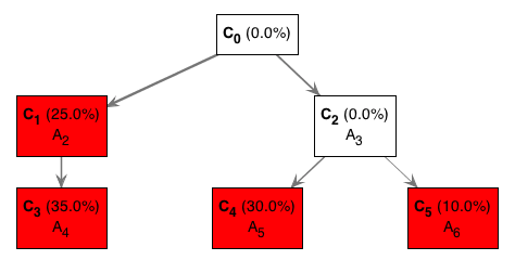
The C₀ represents the aberration-free clone.
The red nodes in the tree indicate the “observed” subclones (C₂, C₄, C₅, C₆) in the tumour sample.
The white boxes represent clones (C₂) that we don’t observe. More on this below.
The mutations each subclone contains is indicated by the mutation identifiers (A₂, A₃, etc).
The percentages represent the portion of the tumour that each subclone represents. The sum of the red boxes should sum to 100%.

How we interpret this tree is as follows:

We started with some aberration-free cells (clone; C₀)
These cells acquired mutation A₂ giving rise to C₁. Independently, another set of cells acquired mutation A₃ giving rise to C₂. In other words, the C₁ cells have mutation A₂ but NOT mutation A₃. Similar logic applies to C₂.
The C₁ cells then acquire mutation A₄ to give rise to C₃. Although not explicitly shown, these C₃ cells have both the mutation A₂ and A₄.
- Not all C₁ cells acquired mutation A₄ though. Hence, why we still observe C₁ cells and why it is shown in a red box.
On the other branch, some C₂ cells then acquire mutation A₅ while others acquire mutation A₆. The C₄ and C₅ have mutation A₃ in addition to the respective mutations they acquired.
- All C₂ cells either acquired mutation A₅ or A_A. We never observe any cells with just mutation _A3. Hence, C₂ appears as a white box and also with 0.0% portion of the tumour.
Ultimately, the tumour consists of 4 observed subclones:
- C₁ with just mutation A₂. This clone accounts for 25% of all tumour cells in the population.
- C₃ with mutations A₂ and A₄. This clone accounts for 35% of all tumour cells in the population.
- C₄ with mutations A₃ and A₅. This clone accounts for 30% of all tumour cells in the population.
- C₅ with mutations A₃ and A₆. This clone accounts for 10% of all tumour cells in the population.

This figure is slightly different from the left half of Figure 1 of the paper:

Left Half of Figure 1

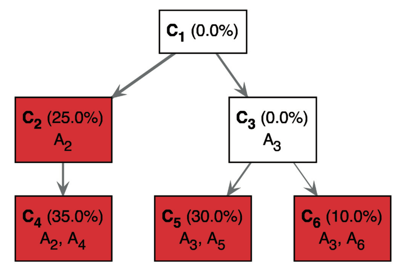
The only difference is that ancestor mutations are “pushed down” to show the complete genotype of each subclone. For instance, it explicitly shows C₄ has having mutations A₂ mutations A₄. While the first tree requires that you make the implicit connection that the descendents cells have the mutations of their parent cells.

Multisample Mode

You can also use TrAp in a multisample mode. This is useful in scenarios where you have multiple samples from the same patient such as a sample before treatment and after treatment. You can leverage the multisample mode to construct trees and compare across them. For instance, the following is the right half of Supplemental Figure S6:

Right Half of Supplemental Figure S6

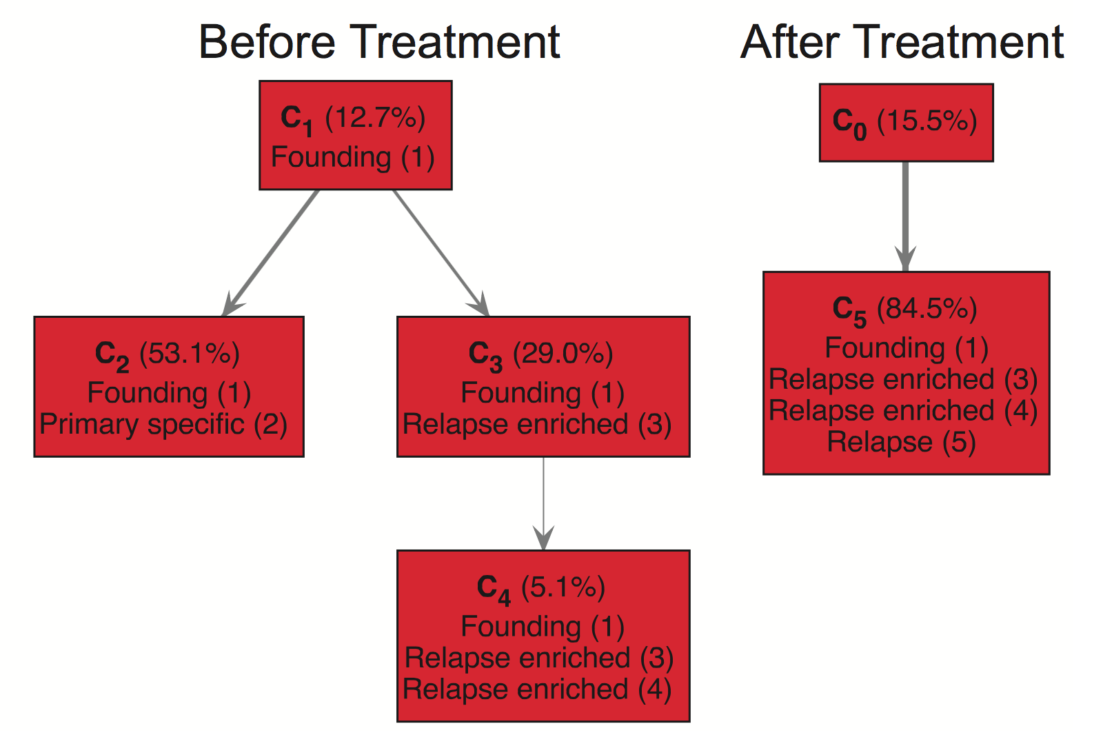
Here we see a “Before Treatment” and an “After Treatment” tree corresponding to two paired samples. This example nicely illustrates how TrAp predicts that subclone C₄ survives treatment and acquires new mutations, Relapse (5), to form the subclone C₅. To use multisample mode, you need to have an input file for each sample. You can see an example of this is in the examples/multisample folder which contains the input files:

fig_s6_1.txt
fig_s6_2.txt
fig_s6_3.txt

The input file format is exactly the same as listed above. The key is each data entry needs to appear in each sample input file with the same identifier. This will allow the multisample mode to match up the data across multiple samples. Then to run, we use the following command:

java -cp TrApWithDependencies.jar multitree.FilterMultiTrees fig_s6_{1..3}.txt

This will end up producing a combined folder with the same contents as single sample mode. The exception is that you will see trees for each sample.

The multisample mode currently only appears to work in version 0.3. If you run it in version 0.31, you will see the following error message:

Error: Could not find or load main class multitree.FilterMultiTrees

Multisample Mode Update

I reported this bug to the developers of TrAp and they have fixed this problem now in version 0.32. You can run multisample mode in version 0.32 like this:

java -cp TrApWithDependencies.jar --multisample fig_s6_{1..3}.txt

Summary

Hope this post helps you get started on constructing phylogenetic trees from your mutation data and interpreting the outputs of TrAp. I would recommend the following references for more information on TrAp: