How "Pseudoalignments" Work in kallisto
@lpachter’s group has recently introduced a new tool called kallisto to the bioinformatics community which marks a huge advancement in how RNA-seq analysis is done. kallisto is a “lightweight algorithm” that is super fast at quantifying the abundance of transcripts from RNA-seq data with high accuracy. The speed of the program can be attributed to the usage of “psuedoalignments” which aims to (from Lior’s blog post):
…determine, for each read, not where in each transcript it aligns, but rather which transcripts it is compatible with…
As such, it’s NOT necessary to do a full alignment of the reads to the genome which is often the slowest step in sequencing analysis. Instead, the raw sequence reads (e.g. fastq) are directly compared to transcript sequences and then used to quanitfy transcript abundance.
How exactly does pseudoalignment work? I spent a bit of time reading the paper (currently in pre-print form at arXiv) trying to understand how kallisto does pseudoalignment and wanted to use this post to share my understanding of the process.
The comparison of the sequencing reads to the transcripts is done using a transcriptome de Bruijn graph (T-DBG) (See this video and Nature primer for a nice explanation of how De Bruijin Graphs can be applied to assembly).
Specifically, the graph is constructed from the k-mers present in an input transcriptome as opposed to reads which is done normally for genome/transcriptome assembly. Here is Figure 1a,b from the paper (modified slightly to reduce complexity):
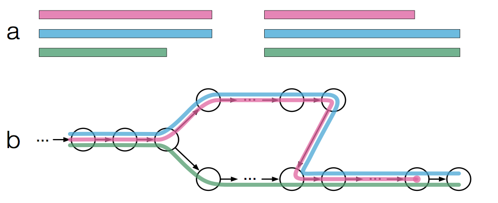
We see in Figure 1a there are three transcripts (pink, blue, and green) which then get converted into a T-DBG (Figure 1b). Each node/vertex is a k-mer in the T-DBG and is associated with a transcript or set of transcripts (represented by the different colors) which is formally described in the paper as a k-compatibility class. In other words, a transcript that contains a node’s k-mer would belong to the k-compatibility class of that node:
In this example, the left most node has a k-compatibility class of all 3 transcripts. While the 3 most top nodes have a k-compatibility class of only the blue and pink transcripts. Once the T-DBG is built, kallisto will then:
store a hash table mapping each k-mer to the contig (linear stretches; e.g. the first 3 nodes) it is contained in, along with the position within the contig. This structure is called the “kallisto index”
If we were to take a read and hash it back to the T-DBG, the different k-mers of the read would be hashed to different nodes in the T-DBG (Figure 1a,c; Modified slighted).
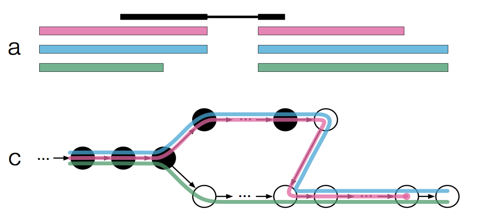
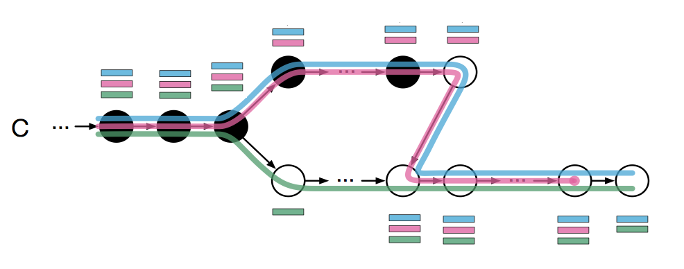
The black nodes represent the k-mers of the read. To find the transcript(s) a read is compatible with, we take the intersection of all k-compatibility classes that a read is associated with; This is formally described as the k-compatibility class of a read (Figure 1c; Modified to add the k-compatibility class of each node).
In this case, the intersection of the k-compatibility classes of all black nodes would be the blue and pink transcripts. This idea can be extended to paired-end reads very easily by simply taking the intersection of the k-compatibility classes along the entire fragment (i.e. both reads).
This is almost what kallisto does except that it takes advantage of the fact that there can be redundant information along a path. For instance, we see that the 3 left most nodes form a contig and all have the same k-compatibility class; This is classified as having the same “equivalence class”. When kallisto hashes a read k-mer to the T-DBG, it looks up the k-compatibility class of the node and then “skips” to the node that is after the last node in the same equivalence class. Figure 1d demonstrates this:

Once the left most k-mer of the read is hashed back, kallisto “skips” the next 2 nodes (as this contains redundant information) and then proceeds to hash only the 4th k-mer of the read. This is quite clever because:
…all k-mers in a contig of the T-DBG have the same k-compatibility class, they will not affect the intersection and therefore looking them up in the hash provides no new information.
So kallisto will always try to “skip over redundant k-mers” or skip to the end of the read. The intersection of the k-compatibility classes then only needs to be done on the “non-skipped” nodes (Figure 1e). This effectively speeds up kallisto since it performs less hash lookups (in this example we only had to perform 3 hash lookups instead of 5). According to the paper:
For the majority of reads, kallisto ends up performing a hash lookup for only two k-mers (Supp. Fig. 6)
I’ve given kallisto (v0.42.3) a spin myself on an RNA-seq library against the Homo_sapiens.GRCh38.rel79.cdna.all.fa.gz transcriptome with --bias and -b 100 parameters:
[quant] fragment length distribution will be estimated from the data
[index] k-mer length: 31
[index] number of targets: 173,259
[index] number of k-mers: 104,344,666
[index] number of equivalence classes: 695,212
[quant] running in paired-end mode
[quant] will process pair 1: fastq/test.1.fastq.gz
                             fastq/test.2.fastq.gz
[quant] finding pseudoalignments for the reads ... done
[quant] learning parameters for sequence specific bias
[quant] processed 92,206,249 reads, 82,446,339 reads pseudoaligned
[quant] estimated average fragment length: 187.018
[   em] quantifying the abundances ... done
[   em] the Expectation-Maximization algorithm ran for 1,521 rounds
[bstrp] number of EM bootstraps complete: 100
The run took just over an hour which is significantly faster than my usual workflow of transcriptome alignment followed by quantification. So it is indeed very fast!
I hope this post helps you understand how pseudoalignment works in kallisto and inspires you to give kallisto a try!